How to Precisely Reduce RO System Operating Cost (2025 Field Guide)

Last updated: November 4, 2025 · Reading time: 12–16 minutes · Audience: plant managers, RO operators, EPCs

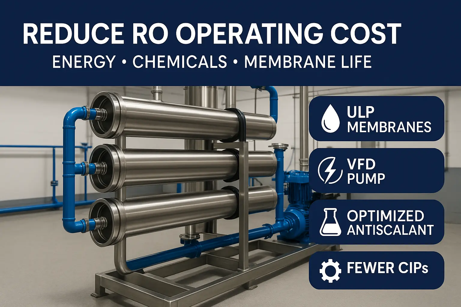
This practical guide shows how to reduce RO operating cost with ultra-low-pressure (ULP) membranes, VFD-controlled high-pressure pumps, dosing optimization, smarter staging and flux, and fewer CIPs—without sacrificing product quality or membrane life. Use the baseline KPIs, checklists, and worked examples to estimate savings and plan a six-week implementation.

Executive Summary — Cost Drivers & Quick Wins

Typical OPEX split for municipal/industrial RO (illustrative ranges): Power 35–60%, Chemicals 10–25%, Membranes 8–15%, Labor 8–12%, Pretreatment/Backwash 5–10%, Concentrate disposal 5–20%. Focus here first to reduce RO operating cost quickly:

1. Swap to ULP membranes (lower net driving pressure at same flux).
2. Add VFD to the high-pressure (HP) pump; control pressure setpoint instead of throttling.
3. Optimize antiscalant/acid dose against limiting salts and LSI/CSI; avoid over-recovery.
4. Increase membrane area (add elements or parallel trains) to run lower flux and pressure.
5. CIP by condition (ΔP/normalized flux) instead of calendar; standardize recipes.

Establish the Baseline — KPIs & Two-Week Audit

Before changing hardware or chemistry, lock in a clean baseline. Track these normalized KPIs daily for two weeks:

• Spezifische Energie (kWh/m³) und specific chemicals (g/m³ by type).
• Normalized flux und ΔP per stage; recovery und availability (% uptime).
• SDI/NTU at RO feed; Temperatur; product EC/pH-Wert.
• CIP frequency, recipe, and chemical per CIP.

Metric	Current	Target after 6 weeks	Anmerkungen
Spezifische Energie	0.85 kWh/m³	0.58–0.65 kWh/m³	ULP + VFD
Antiscalant dose	4.0 mg/L	3.0–3.5 mg/L	Re-model dose vs recovery
CIP frequency	1× / month	1× / 6–8 weeks	Condition-based triggers
Normalized ΔP	+12%/month	<+4%/month	Flux & pretreatment tuning

Energy Reduction Tactics

1) Ultra-Low-Pressure (ULP) Membranes

ULP elements deliver target flux at lower pressure, cutting pump power instantly. Plants moving from 1.3–1.5 MPa to ~0.8–1.0 MPa typically see ≈25–35% energy reduction at equal recovery and temperature. Validate with a trial skid and normalize for temperature.

2) VFD on the High-Pressure Pump

A variable-frequency drive controls discharge pressure without throttling losses, enables soft start, and moderates water hammer. ≈10–20% annual energy savings are common and you gain better process stability.

3) Increase Membrane Area (More Elements / Parallel Trains)

More area → lower flux at the same production → lower required pressure and slower fouling. The combination often reduces ΔP slope and extends element life by 6–12 months.

4) Staging & Recovery Tuning

Over-recovery drives osmotic pressure and ΔP up. Tune recovery and, where justified, use interstage boosters only after a cost–benefit check. The best way to reduce RO operating cost is often a few percent less recovery with fewer CIPs and lower pressure.

Chemical Cost Optimization

5) Antiscalant Dose Optimization

• Model dose from water analysis and recovery; target the limiting salts (CaCO₃/CaSO₄/BaSO₄/SiO₂).
• Run a 2–3 level dose trial (e.g., 3.0 / 3.5 / 4.0 mg/L) and trend ΔP and normalized flux.
• Expect ~15–25% chemical savings with no loss of stability.

When carbonates dominate, a small acidification can reduce dose further; avoid CaSO₄ risk when using H₂SO₄.

6) CIP by Condition, Not Calendar

• Trigger by normalized flux loss (e.g., −10%) oder ΔP rise (e.g., +15–20%).
• Standardize acid/alkali recipes and soak times; record chemical per CIP and recovery time.
• Check that pre-CIP permeate EC and SDI are still on spec; if not, tackle pretreatment first.

7) Permeate Post-Treatment Optimization

For neutralization (NaOH) and optional CO₂ degassing, size from CO₂ load and target pH; trim dosing to avoid overshoot and wasted caustic.

Membrane Technology Choices

• Anti-fouling (AF) membranes: smoother surface/coatings improve cleanability and reduce CIP frequency.
• Element lifetime planning: 2–3 years typical under good control; premature replacement inflates OPEX and CapEx.
• Max operating temperature: keep ≤35–40 °C for longevity; observe vendor limits for continuous vs. CIP exposure.

Pretreatment & Operating Environment

• Dechlorination & metals control: protect polyamide from oxidants; prevent Fe/Al carryover that seeds fouling.
• SDI/NTU targets: lower SDI extends run length and reduces CIP chemical spend.
• Filtration & backwash optimization: ensure adequate velocity and air scour; log backwash water and energy.
• Instrumentierung: verify meters (kWh, flow), pressure sensors, pH/ORP are accurate; poor metering hides savings.

Worked Savings Scenarios (Replace with Your Data)

Scenario A — ULP Retrofit + VFD

Plant 1,000 m³/d, baseline 0.85 kWh/m³. After ULP and VFD pressure control: 0.58 kWh/m³ (−32%). At $0.12/kWh, annual energy saving ≈ $118,000. Payback for membranes + VFD: ≈ 8–14 months depending on pricing.

Scenario B — Antiscalant Re-model + Hybrid Acid Assist

Dose reduced from 4.0 → 3.0 mg/L (−25%); slight feed acidification keeps LSI ≤ 0. ΔP slope halves; CIP reduced by one event/quarter. Chemical saving and downtime saving together cut OPEX by 8–12%.

Scenario C — Add One Element per Vessel

Per-element flux −15% and pressure −8–12%; energy −8–10% and membrane life +6–12 months. Check pump curve and NPSH before approval.

Six-Week Implementation Roadmap

1. Week 1–2: KPI audit; instrument verification; safety review; confirm membrane/pump limits.
2. Week 3–4: VFD trial curve; antiscalant re-model and A/B dose test; recovery/flux tuning; SOP drafts.
3. Week 5–6: Pilot ULP/AF skid; finalize CIP triggers; update LCC/OPEX dashboard; operator training.

Visuals & Downloadables

• Baseline KPI & OPEX template (XLSX)
• Reverse Osmosis Solutions - Case Studies - Request an Audit
• Hintergrundlektüre: EPA Water Research - ISO Water Quality

Request a Cost-Cut Plan

Upload 6–8 weeks of kWh, chemical dosing, ΔP/flux, recovery, and temperature data. We’ll return a customized plan to reduce RO operating cost with expected savings and payback.

Talk to an Engineer

About the Author

Stark Water — Process engineers focused on RO/NF, energy optimization, and lifecycle cost control. We design, pilot, and operate plants worldwide.

FAQs — Reduce RO Operating Cost

1) How much can ULP membranes save vs. standard elements?

Field results frequently show 25–35% energy reduction at similar recovery and temperature. Validate with a pilot and pump curve check.

2) VFD or control valve — which saves more power?

A VFD eliminates throttling losses and follows a pressure setpoint, typically saving 10–20% energy with better ramping and less water hammer.

3) How do I choose between acid dosing and antiscalant only?

If carbonate is the limiting scale, mild acidification plus a leaner antiscalant dose can minimize cost. Always check CaSO₄/silica indices.

4) What SDI/NTU targets reduce CIP frequency?

Lower SDI/NTU correlates with slower ΔP rise. Optimize filter backwash and coagulant to keep SDI down and extend run length.

5) AF vs. standard elements for seasonal feeds?

AF membranes are more forgiving and often clean faster, reducing CIP cost; verify compatibility with your CIP recipes and oxidant control.

6) What’s a safe maximum operating temperature for RO?

Most polyamide elements run best ≤35–40 °C continuously; check your vendor’s datasheet and adjust flux/pressure accordingly.

7) How do I track normalized performance correctly?

Use temperature-corrected flux and pressure; trend ΔP and recovery with alarms to trigger condition-based CIP windows.